 Casting simulation
JoseCast Analyzer
See inside the part before you pour it. Filling and solidification simulation for steel, stainless steel and cast iron. Free for life.

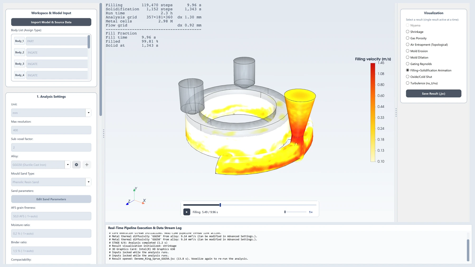
Catch scrap on the screen
The real value of a simulation is the right decision it lets you make before anything is poured.
See defects before you pour
See the risk of shrinkage, porosity, air entrapment and cold shuts on the model, before the mould is even made.
Fewer trial castings
Test the gating and riser design on screen, and go to the foundry with a more mature design.
Decide with data
Ten result fields and the filling–solidification animation base the engineer's decision on numbers and images.
From the STEP model to the casting result
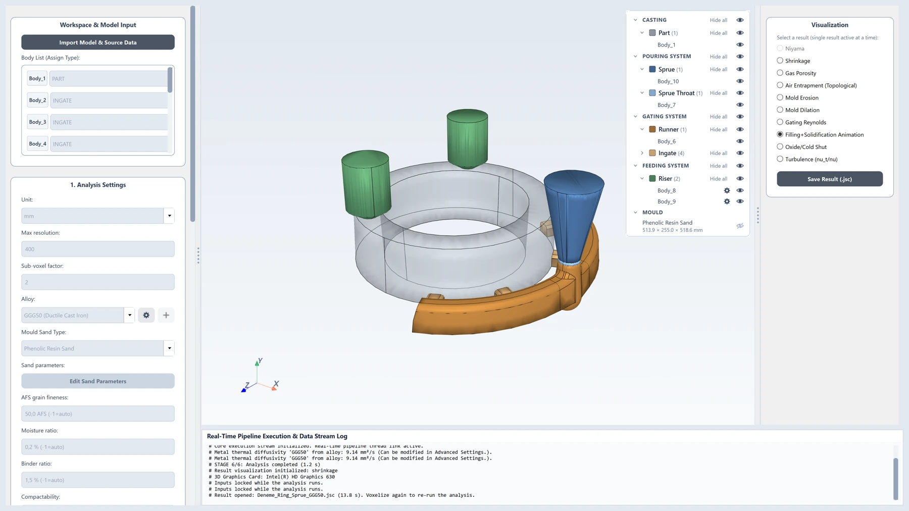
Load the STEP file, assign a casting element type to each body (part, feeder, ingate, runner, sprue, pouring basin, core, chill…), and choose the alloy and the mould material. The program solves the stages in order: filling first, then solidification once filling is complete.
JoseCast AnalyzerSTEP → 3DFilling
Flow of the liquid metal from the pouring basin into the cavity, the free surface and air pockets. If switched off, the fill time and the cooling during filling are calculated from relations in the casting literature.
Solidification
After filling: temperature, solid fraction and the solidification time of every point in the metal and the mould. The heat lost during filling is accounted for by an energy balance. Eutectic plateau in cast iron.
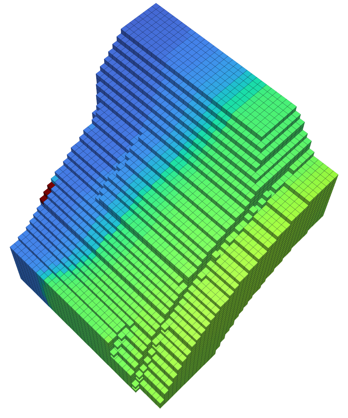
It all starts with a cube.
Casting is governed by differential equations: metal flow by the Navier–Stokes equations, heat spreading by the heat conduction equation, solidification by the enthalpy equation. Analyzer solves these equations on cubes (voxels) that fill the part and the mould. Each cube is a control volume: the mass and energy entering, leaving and accumulating in it are computed one by one. A regular cubic grid is the structure on which computational fluid dynamics solves these equations most robustly and accurately.
- Conservation, exactly
The six faces of a cube are axis-aligned, so the flux between neighbouring cubes is computed exactly. Mass and heat leaving one cube enter its neighbour in full, and the total is conserved to machine precision.
- A natural fit for the flow method
The lattice Boltzmann method is defined on a regular lattice: flow is streamed from each cube to its neighbours in 19 fixed directions. The cubic grid is the method's own language; no conversion or approximation is needed.
- No meshing, every STEP works
There is no triangle or tetrahedral mesh to build, repair and quality-check. Voxelisation works equally robustly on every CAD model, and a grid fine enough to put at least three cells across the thinnest wall is chosen automatically.
- Fine in the part, smart in the mould
The metal is solved on uniform cubes, the mould on cubes that are fine near the metal and coarse further away (octree). Accuracy stays in the metal and computing effort is not wasted in the sand; the wall position is found more precisely than the cube step with a sub-voxel distance field.
Triangle mesh or cubes?
Many programs solve the equations on a triangle or tetrahedral mesh derived from the part surface. We deliberately chose cubes.
| Triangle / tetrahedral mesh | JoseCast: cubes + octree | |
|---|---|---|
| Preparation | Mesh generation, repair and quality checks; can take hours on a complex part | Automatic and robust for every STEP; no manual meshing |
| Imperfect geometry | Open edges, intersecting faces or sliver triangles break the mesh and the solution | Inside/outside decided by ray test; small surface defects do not spoil the result |
| Numerical stability | Flat and distorted elements worsen the error and the time step | Every cell has the same shape; there is no such thing as a bad element |
| Conservation | Flux on skewed faces stays approximate | Exact flux on axis-aligned faces; mass and energy are conserved |
| Parallel speed | Irregular memory access | Regular memory; every processor core works efficiently |
We use the triangle surface mesh only to read the STEP geometry; the equations are solved on cubes.
Six steps from STEP to result
Every step rests on a published method; the sources are on the Literature page.
- 01
Voxelisation
A ray is cast through the centre of each cell; how many times it crosses the CAD surface tells whether the cell lies inside the part. A thin-wall rule refines the grid automatically; embedded cores and chills are not overwritten by the part.
Möller–Trumbore ray test · Δx ≤ t_min / 3 - 02
Mould and octree
The mould is built by cutting the part's real surface out of the mould box with a Boolean operation: real geometry, not estimated empty cells. The sand is divided into cubes that are fine near the metal and coarse further away; accuracy stays next to the metal while the computing effort drops many times over.
Boolean cut · octree (fine near the metal, coarse far away) - 03
Filling
Metal really flows from the pouring basin under hydrostatic pressure. The free surface is tracked cell by cell, the turbulent boundary layer at the wall is modelled, and thin sections are solved automatically on a grid twice as fine. Mass is conserved to machine precision.
Free-surface lattice Boltzmann (D3Q19) · Spalding wall model - 04
Air and gas
Air pockets trapped in the metal push back with their own pressure; the air leaks out through the sand, and in green sand the moisture steam is taken into account too.
Ideal-gas pockets · Darcy leakage + Klinkenberg correction - 05
Solidification
The heat solution starts when filling is complete; metal, mould, cores, chills and sleeves are solved in a single system. Scheil curve in steel, eutectic latent heat plateau in cast iron; exothermic sleeves produce real heat.
Implicit finite volume on the octree · Voller–Swaminathan enthalpy method - 06
Result fields
The Niyama family, feeding path, shrinkage, gas, oxide, erosion and mould dilation all come from the same solution.
Niyama / Carlson–Beckermann · Dijkstra
Five alloy families, each with its own physics
We do not add families we cannot validate; each family has its own solidification and shrinkage path. You can add your own alloy from its chemical analysis with CALPHAD.
Ten result fields, one 3D interface
Every result is shown as a coloured field on the part; filling and solidification can be followed as an animation.
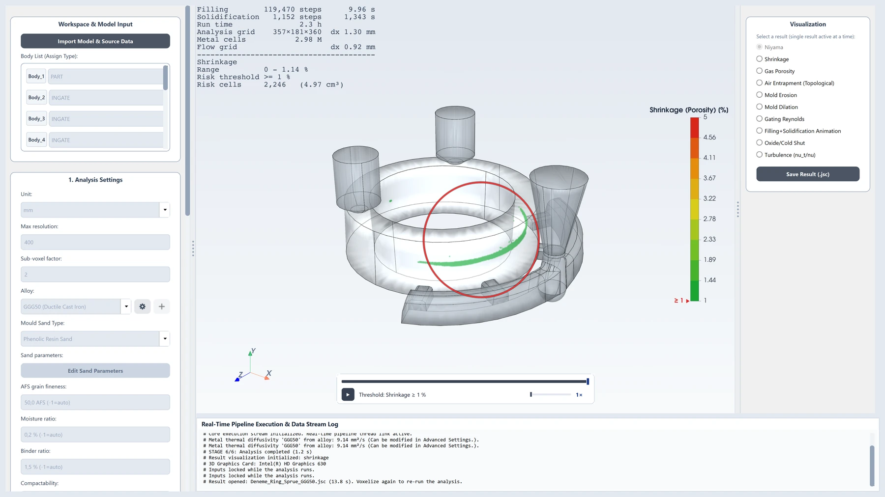
Micro-shrinkage risk in steel and stainless steel from the temperature gradient and the cooling rate.
Shrinkage cavities that may form in regions that cannot be fed.
The risk of gas-related porosity.
Air pockets trapped inside the metal during filling.
Where cooling metal fronts meet, with a risk of oxides and cold shuts.
Regions where fast-flowing metal erodes the mould surface.
Swelling of the mould wall under metal pressure.
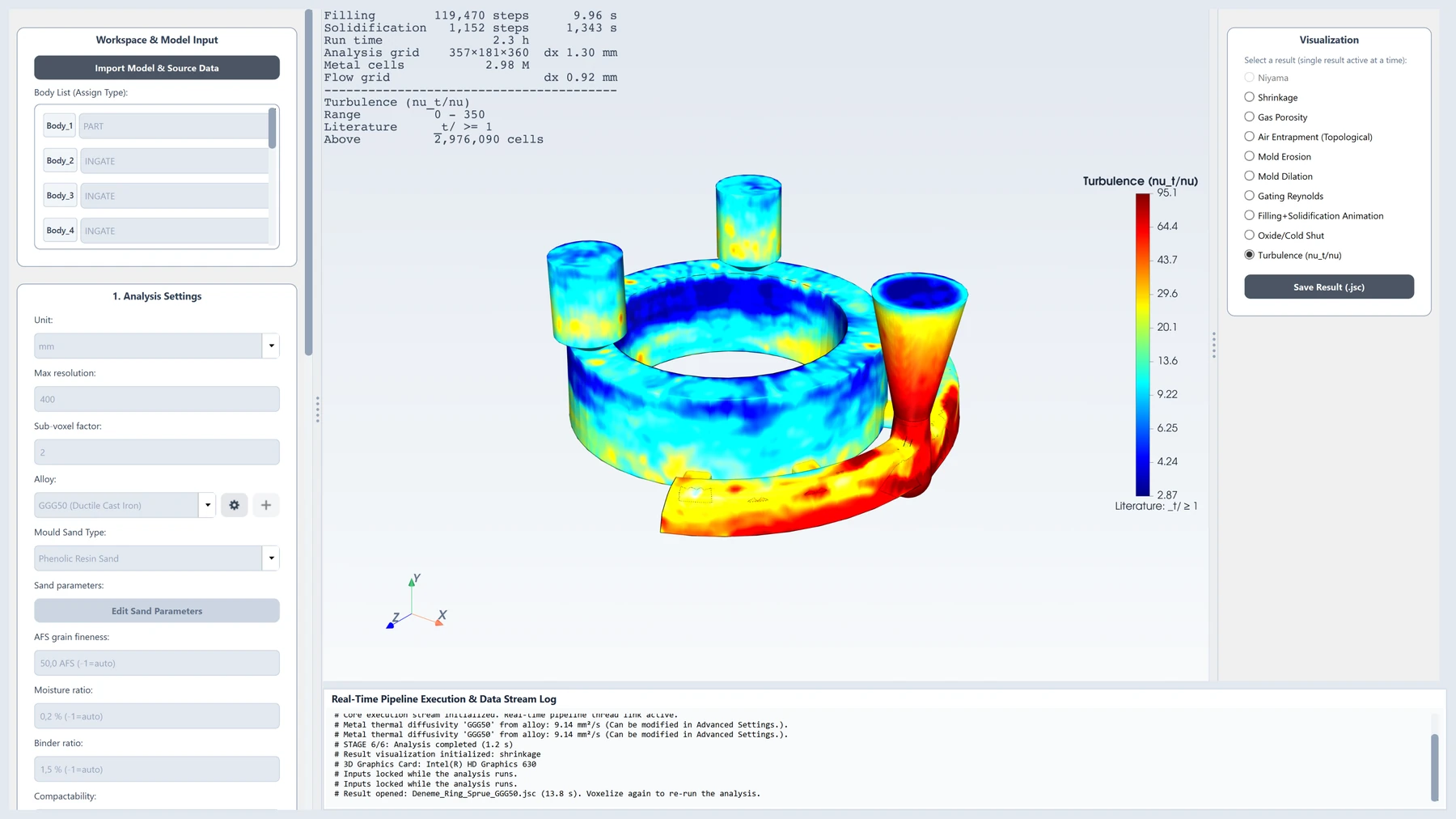
Regions of turbulent flow during filling.
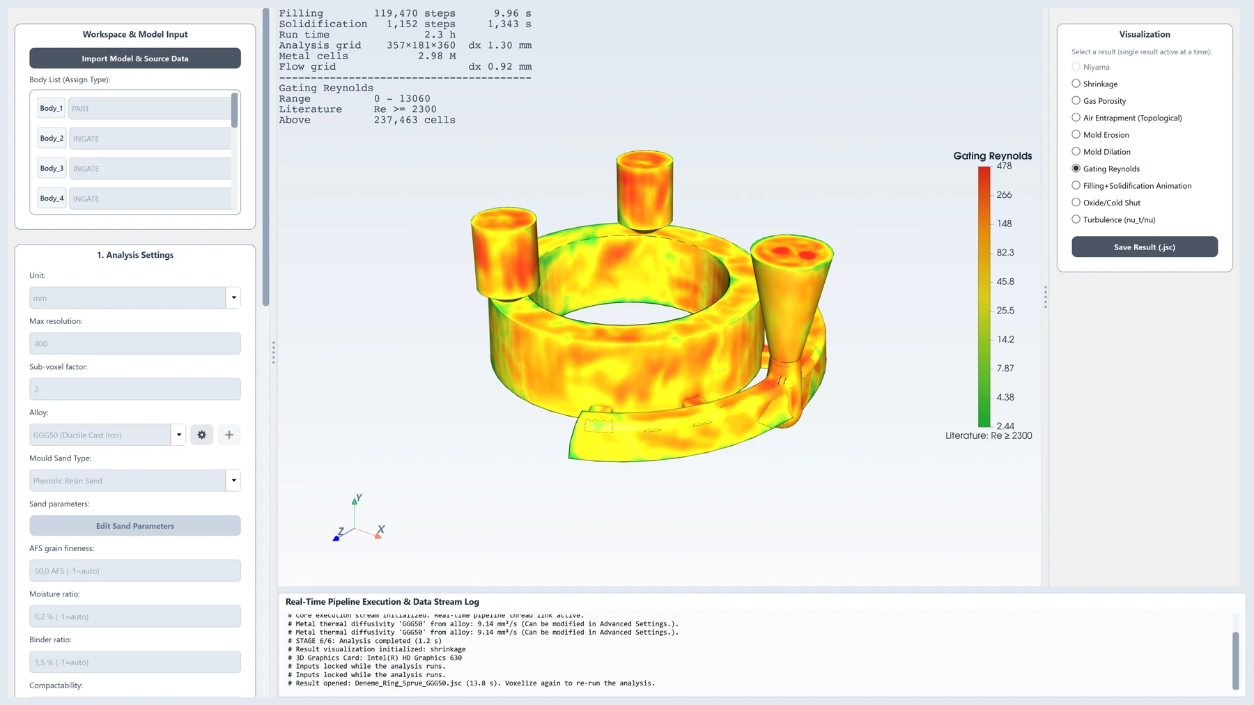
The flow regime in the runners and ingates.
Follow filling and solidification step by step.
What is it built for?
Analyzer is deliberately narrow and deep: we do not add materials and processes we cannot validate.
- Steel, stainless steel and cast iron alloys
- Sand moulds, gravity pouring
- The whole result is stored in a single result package (.jsc) and can be reopened; the solver runs in a separate process, so the analysis continues if the interface closes
- The interface is in English only; the program has no other language option
For a simulation you can trust
A simulation is worth as much as you can trust its result. That is why we build Analyzer around a few strict rules.
No number without a source
Every coefficient is either sourced or a clearly marked assumption. If it is neither, the program gives a clear error.
It analyses, it does not design
The program shows the result; placing risers or chills is left to the engineer.
One thermal solution
Metal, mould, cores and chills are solved in a single linear system; heat passes between them without loss.
Real geometry
The model is read from the STEP file; the mould is solved on an octree grid, fine near the part and coarse further away.
Your data stays with you
The simulation runs entirely on your computer; your model and results are not sent anywhere.
No fallbacks in the display
If a result field was not calculated, nothing estimated is shown; the field stays grey and the reason is stated.
The JoseCast Analyzer interface
The program's own screens, from loading the model to the result fields. The interface is in English.
See JoseCast Analyzer at work
An introduction video taking a part step by step from its STEP file to the simulation result.
Download JoseCast Analyzer for free
Install from the Microsoft Store or download the installer directly. Both give you the same program, and both are free for life.
The Microsoft Store version is signed by Microsoft and updates itself. If Windows shows a warning when the directly downloaded version first starts, choose "More info" and then "Run anyway".